
Machine Learning Project: Moving Car Detection Using GMM and SVMs
Introduction
This project develops an application to detect moving car on high way, and thus computing car’s speed basing on an input video. In particular, this work applies GMM model [1] to detect moving objects that could consist moving cars or objects likely trees, motors. Next, Support Vector Machine (SVM) is applied to classify between observed car and the others, and eventually the speed of car is computed. This project uses Python and OpenCV library to count cars, trained a classifier with the set of vehicle and non-vehicle images. The source video file section used for this project is from Highway 01 - Free Video Footage - Background HD Free.
To accomplish this, I have done the following:
- Training the Linear Support Vector Machine to classify the vehicle and non-vehicle objects using Histogram of Oriented Gradients (HOG).
- Opening the video file and applying Gaussian Mixture Model to isolate the moving objects from a static background.
- Classifying the vehicle object by using the trained SVMs.
- Tracking the cars and computing the speed of the car.
Histogram of Oriented Gradients:
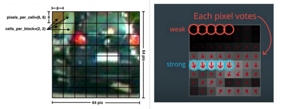
A class of object such as a vehicle vary so much in color. Structural cues like shape give a more robust representation. Gradients of specific regions directions captures some notion of shape. The idea of HOG is instead of using each individual gradient direction of each individual pixel of an image, the pixels are grouped into small cells. For each cell, all the gradient directions are computed and grouped into a number of orientation bins. The gradient magnitude is then summed up in each sample. So stronger gradients contribute more weight to their bins, and effects of small random orientations due to noise is reduced. This histogram gives a picture of the dominant orientation of that cell. Doing this for all cells gives a representation of the structure of the image. The HOG features keep the representation of an object distinct but also allow for some variations in shape.
Feature Extraction:
The number of orientations, pixels_per_cell, and cells_per_block for computing the HOG features of a single channel of an image can be specified. The number of orientations is the number of orientation bins that the gradients of the pixels of each cell will be split up in the histogram. The pixels_per_cell is the number of pixels of each row and column per cell over each gradient the histogram is computed. The cells_per_block specifies the local area over which the histogram counts in a given cell will be normalized. Having this parameters is said to generally lead to a more robust feature set.
feature_params = {
'color_model': 'yuv', # hls, hsv, yuv, ycrcb
'bounding_box_size': 64, # 64 pixels x 64 pixel image
'number_of_orientations': 11, # 6 - 12
'pixels_per_cell': 8, # 8, 16
'cells_per_block': 2, # 1, 2
'do_transform_sqrt': True
}
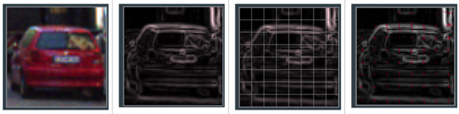
source = FeatureSourcer(feature_params, vehicle_image)
vehicle_features = source.features(vehicle_image)
rgb_img, y_img, u_img, v_img = source.visualize()
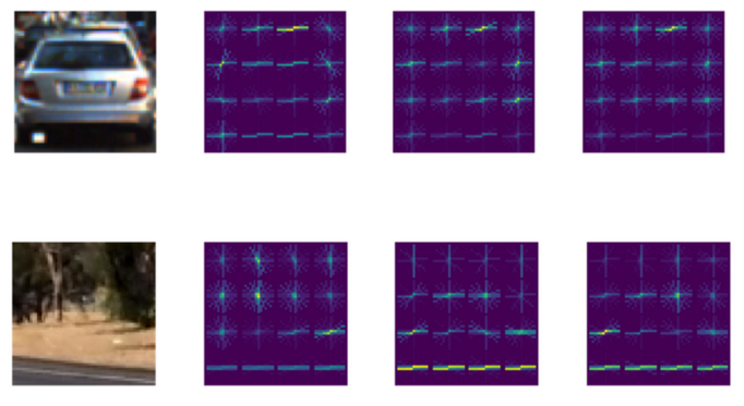
Classifier Training:
The Support Vector Machine model is trained by using 8792 samples of vehicle images and 8968 samples of non-image. This dataset is preselected by Udacity with images from the GTI vehicle image database and the KTTI vision benchmark suite. As a safety measure, a scaler is used to transform the raw features before feeding them to the classifier for training, reducing the chance of the classifier to behave badly.
    # Feature Extraction...
    for img in vehicle_imgs:
      vehicles_features.append(source.features(img))
    for img in nonvehicle_imgs:
      nonvehicles_features.append(source.features(img))

    # Scaling Features...
    unscaled_x = np.vstack((vehicles_features, nonvehicles_features)).astype(np.float64)
    scaler = StandardScaler().fit(unscaled_x)
    x = scaler.transform(unscaled_x)
    y = np.hstack((np.ones(total_vehicles), np.zeros(total_nonvehicles)))

    # Training Features...
    x_train, x_test, y_train, y_test = train_test_split(x, y, test_size = 0.2, random_state = rand.randint(1, 100))
    svc = LinearSVC()
    svc.fit(x_train, y_train)
    accuracy = svc.score(x_test, y_test)
Importing the input video:
The first step to counting cars is to import the necessary libraries. Numpy library is used for creating vectors and matrices, OpenCV is used for reading and manipulating the image, and Pandas is used for keeping the data in an organized manner. The next step is to open the video file named traffic.mp4 which is done with cv2.VideoCapture(). Next, the pertinent information about the video is acquired such as the total amount of frames (frames_count), the frames per second (fps), the width of the video (width), and height of the video (height). The width and height variables will later be used as integers int() to adjust the location of the images on the screen.
A dataframe is created with the Pandas library where the number of rows equals the total amount frames in the video. This dataframe will be used to keep the car tracking data organized where new columns are added as new cars are detected in the video. Traking object is done by using counters or empty lists. The background subtractor is created in cv2.createBackgroundSubtractorMOG2() that is one of the most important parts of this script as this helps isolate the moving objects from a static background. Each pixel in the frame was compared with model formed from GMM. Pixels with similarity values under the standard deviation and highest weight factor were considered as background, while pixels with higher standard deviation and lower weight factor considered as foreground. The background subtractor works well on videos that have a static background but a video with a background that is not stationary would most likely use different methods for isolating key objects. One such method is using HSV Color Filtering which can be seen in the Python OpenCV Juggle Counter tutorial.
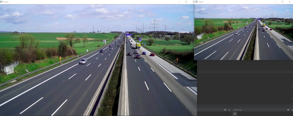
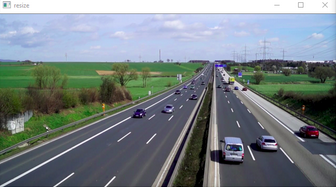
The ratio variable is used to resize the image in order to reduce lag. The while True: loop starting keeps displaying each video frame after another if ret: is true ( if a frame gets captured) otherwise it breaks out of the loop and stops the video. Each frame is resized to reduce lag. The video frames are displayed with cv2.imshow(“WINDOWNAME”, FRAMENAME). The original and reduced size of the frame can be seen below. It is also useful to resize the image if it takes up too much space on the screen.
   import numpy as np
   import cv2
   import pandas as pd

   cap = cv2.VideoCapture('traffic.mp4')
   frames_count, fps, width, height = cap.get(cv2.CAP_PROP_FRAME_COUNT), cap.get(cv2.CAP_PROP_FPS), cap.get(
       cv2.CAP_PROP_FRAME_WIDTH), cap.get(cv2.CAP_PROP_FRAME_HEIGHT)
   width = int(width)
   height = int(height)
   print(frames_count, fps, width, height)

   # creates a pandas data frame with the number of rows the same length as frame count
   df = pd.DataFrame(index=range(int(frames_count)))
   df.index.name = "Frames"

   framenumber = 0  # keeps track of current frame
   carscrossedup = 0  # keeps track of cars that crossed up
   carscrosseddown = 0  # keeps track of cars that crossed down
   carids = []  # blank list to add car ids
   caridscrossed = []  # blank list to add car ids that have crossed
   totalcars = 0  # keeps track of total cars

   fgbg = cv2.createBackgroundSubtractorMOG2()  # create background subtractor

   while True:

       ret, frame = cap.read()  # import image

       if ret:  # if there is a frame continue with code

           image = cv2.resize(frame, (0, 0), None, ratio, ratio)  # resize image
Applying Thresholds and Transformations:
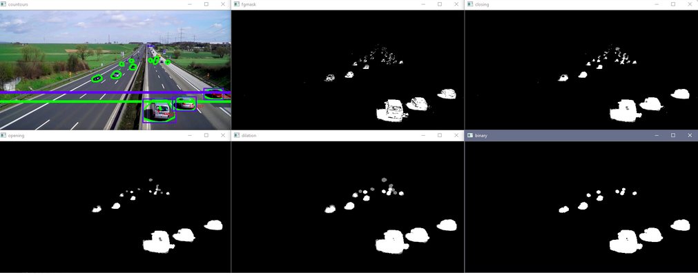
The next important step to counting cars is to apply thresholds and transformations to the image to allow better isolation of moving objects. Firstly, the image is converted to gray scale for better analysis and then is applied the background subtractor to distinguish moving objects. The top left image below is the unaltered frame and the top middle image is the frame with background subtractor applied. As one can see, OpenCV was able to distinguish the moving cars from the static background. However, the background subtractor is not perfect and needs some transformations done to it to try and better isolate the moving cars.
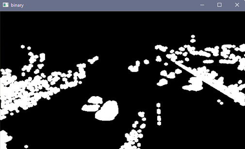
The functions in first four lines of the code below isolate the cars into shapes that can be more easily tracked. First line states the type and size of the kernel which adjusts the image according to the morphological transformations. The ‘shadows’ are removed from the transformations (the gray portions) to better isolate the cars. The main point of applying these transformations is to remove noise, isolate the cars, and make them into solid shapes that can be more easily tracked. The binary image bins in the bottom right corner will be used to create contours around the cars in the next section. Here are some links for more information on morphological transformations and the kernel.
gray = cv2.cvtColor(image, cv2.COLOR_BGR2GRAY) # converts image to gray
fgmask = fgbg.apply(gray) # uses the background subtraction
# applies different thresholds to fgmask to try and isolate cars
# just have to keep playing around with settings until cars are easily identifiable
kernel = cv2.getStructuringElement(cv2.MORPH_ELLIPSE, (5, 5)) # kernel to apply to the morphology
closing = cv2.morphologyEx(fgmask, cv2.MORPH_CLOSE, kernel)
opening = cv2.morphologyEx(closing, cv2.MORPH_OPEN, kernel)
dilation = cv2.dilate(opening, kernel)
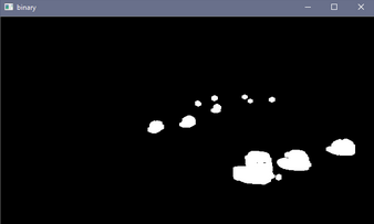
retvalbin, bins = cv2.threshold(dilation, 220, 255, cv2.THRESH_BINARY) # removes the shadows
By applying trained SVM model using extrated HOG feature, now that the cars are better isolated.
Creating Contours and Acquiring Centroids:
Firstly, the contours are draws around the isolated cars. The horizontal lines in the image below are created. The blue line is used later on in the code to indicate when to start and stop keeping track of the contours as we are only interested in contours that are well defined. As seen in the top left image below, the car contours in the distance start merging and becoming indistinguishable from other car contours which increases the difficulty in differentiating one car from another. Anything above the blue line ([x,y] zero position is top left corner of image) isn’t kept track of but anything below is. The green line is used later on in the code to keep track of whether the car is moving upwards or downwards by checking if the car passes the line when compared to the previous frame. This will be explained later on.
There are the minimum and maximum area values that allow a contour to be counted. The loop in the code below loops through all the contours and filters out contours that do not meet certain criteria. The first criteria is that the contour must be the parent contour, that is, it cannot be within another contour. This is important because sometimes small contours are within other contours due to the transformations applied earlier not eliminating every imperfection. This is eliminating any contour that is within any contour; a car cannot be within another car. The area acquired of the contour is checked to see if it is within an acceptable size. This removes any contours that are too small such as noise or too large such as a big object that is not a car. The x and y position of the contour’s centroid are acquired to check if the car is below the blue line and keeps track of it as these contours are more distinguishable than the ones in the far off distance. If the centroid of the contour passes all of these criteria, then a blue box is created around the outer bounds of the contour, the centroid text is labeled, a marker is created, and the x and y positions of the centroid are added to the vector created earlier. Ii will then extract all the non-zero entries in the centroid vectors.
    # creates contours
        im2, contours, hierarchy = cv2.findContours(bins, cv2.RETR_TREE, cv2.CHAIN_APPROX_SIMPLE)

        # use convex hull to create polygon around contours
        hull = [cv2.convexHull(c) for c in contours]

        # draw contours
        cv2.drawContours(image, hull, -1, (0, 255, 0), 3)

        # line created to stop counting contours, needed as cars in distance become one big contour
        lineypos = 225
        cv2.line(image, (0, lineypos), (width, lineypos), (255, 0, 0), 5)

        # line y position created to count contours
        lineypos2 = 250
        cv2.line(image, (0, lineypos2), (width, lineypos2), (0, 255, 0), 5)

        # min area for contours in case a bunch of small noise contours are created
        minarea = 300

        # max area for contours, can be quite large for buses
        maxarea = 50000

        # vectors for the x and y locations of contour centroids in current frame
        cxx = np.zeros(len(contours))
        cyy = np.zeros(len(contours))

        for i in range(len(contours)):  # cycles through all contours in current frame

            if hierarchy[0, i, 3] == -1:  # using hierarchy to only count parent contours (contours not within others)

                area = cv2.contourArea(contours[i])  # area of contour

                if minarea < area < maxarea:  # area threshold for contour

                    # calculating centroids of contours
                    cnt = contours[i]
                    M = cv2.moments(cnt)
                    cx = int(M['m10'] / M['m00'])
                    cy = int(M['m01'] / M['m00'])

                    if cy > lineypos:  # filters out contours that are above line (y starts at top)

                        # gets bounding points of contour to create rectangle
                        # x,y is top left corner and w,h is width and height
                        x, y, w, h = cv2.boundingRect(cnt)

                        # creates a rectangle around contour
                        cv2.rectangle(image, (x, y), (x + w, y + h), (255, 0, 0), 2)

                        # Prints centroid text in order to double check later on
                        cv2.putText(image, str(cx) + "," + str(cy), (cx + 10, cy + 10), cv2.FONT_HERSHEY_SIMPLEX,
                                    .3, (0, 0, 255), 1)

                        cv2.drawMarker(image, (cx, cy), (0, 0, 255), cv2.MARKER_STAR, markerSize=5, thickness=1,
                                       line_type=cv2.LINE_AA)

                        # adds centroids that passed previous criteria to centroid list
                        cxx[i] = cx
                        cyy[i] = cy

        # eliminates zero entries (centroids that were not added)
        cxx = cxx[cxx != 0]
        cyy = cyy[cyy != 0]
Traking Cars:
The section of the script below is responsible for keeping track of the cars in the video. The method used for keeping track of the cars is to check which x and y centroid position pair in the current frame is closest to another x and y centroid position pair in the previous frame. This works great for this application since the contours are large and spaced out but can cause an issue when the contours are small and in close proximity with a low frame rate.
An empty list is created that will be used later on for the indices of the centroids in the current frame that are added to centroids in the previous frame. The if statement below is the algorithm that keeps track of the cars. The first if statement if len(cxx) checks if there are any centroids in the current frame that have passed the criteria mentioned in the section above. If there are centroids that have passed the criteria, then the rest of the if statement can commence in order to start tracking cars.
The next if statement if not car-ids checks if the empty list car-ids created is indeed empty. This is used to check if there have not been any cars recorded yet. If there have not been any cars recorded yet, then there will be a loop loops through all the current centroids that have passed the criteria and creates car-ids to start keeping track of cars. The new car-ids are appended to the empty car-id list and a new car-id column is added to the dataframe. The car-ids corresponding x and y centroid position are added to the dataframe for that specific frame row (framenumber) and carid column (carids). Finally, the totalcars counter increases the total car count.

Now, the speed of the car can be calculated since the time and the distance between two lines are already known.
Conclusions:
The project is conducted using data of vehicle images and non-vehicle images to train a classifier that helps detect cars and the other objects. The detection moving object uses Gaussian Mixture model method as well as SVM model to classify cars among others and the tracking object uses Euclide distance of the centroid between current and previous frame. The common issues could be arisen in this project if the maximum radius is too large and multiple centroids are close to other centroids.