Machine Learning Project: Acoustic Scene Classification Using A Deeper Training Method for Convolution Neural Networks

Introduction

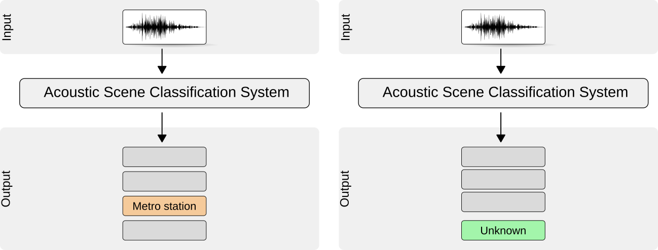
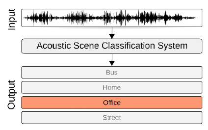
Acoustic scene classification (ASC), aiming to categorize the types of locations where a sound was recorded, represents one of the main tasks of a recently appearing research field named “machine hearing”[1]. By exploiting information extracted from the soundscape, ASC is explored in various applications such as context-aware services[2], audio archive management[3], and intelligent wearable devices[4]. The most challenge of this task is that a recording related to a given location can contain various sound events. A well-learned model, therefore, should not only focus on performing either background or foreground sounds. Additionally, concerned issues may come from datasets that show different class numbers, recording conditions, biased recording time, making it the most challenging task in the sound recognition area[5]. Hence, recent studies have dedicated to propose various methods for ASC task, and deep learning approach has recently proven effectively[6].

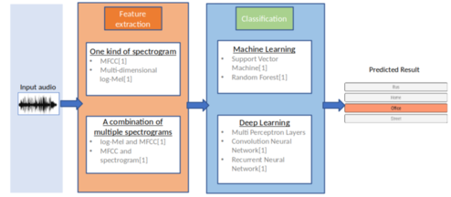
For the front-end extracted feature considered as one main step of an ASC model, mel-frequency cepstral coefficients (MFCC) has widely applied to the research of speech firstly explored in ASC[8]-[11]. Some did experiments on linear predictive coefficients (LPCs) to calculate a power spectrum of the signal[12]. However, acoustic scenes are less structured than speech signals explaining why the mentioned techniques have not shown efficiency. To address this problem, spectrogram features inspired from researches on image processing has recently employed in [14].

Regarding back-end learning models, conventional classifiers, which proved effectively on speech signals such as Gaussian mixture models (GMMs)[8], support vector machines (SVMs)[15], and hidden Markov models (HMMs)[16], were firstly exploited over the ASC task. However, deep learning techniques have recently become a trend for the ASC task[17] and have proved much more effectively [7]. Convolutional Neural Networks (CNNs) [18] are considered as the most effective classification for ASC tasks, which were early applied [19] and has be shown to be an effective approach. To enhance the classifier, various data augmentation techniques have been approached.

Inspired by the aforementioned techniques, this project, therefore, invokes Gammatone filters [22] to transform audio segments into time-frequency shape before feeding into the back-end classification. A baseline proposal based on CNNs is then introduced. Thus, motivated from the transform learning technique proposed in [23], a training process that forces the baseline learning the middle convolutional layer deeper is proposed. This work also applies a data augmentation named mixup that is useful to improve the model’s performance. To evaluate the performance of the proposed method with different neural networks, the project conducted extensive experiments over DCASE2016 task 1A dataset [24]. The experiments demonstrate that my architecture outperforms the conventional models such as GMM, SVMs as well as DCASE2016 baseline.

System Description

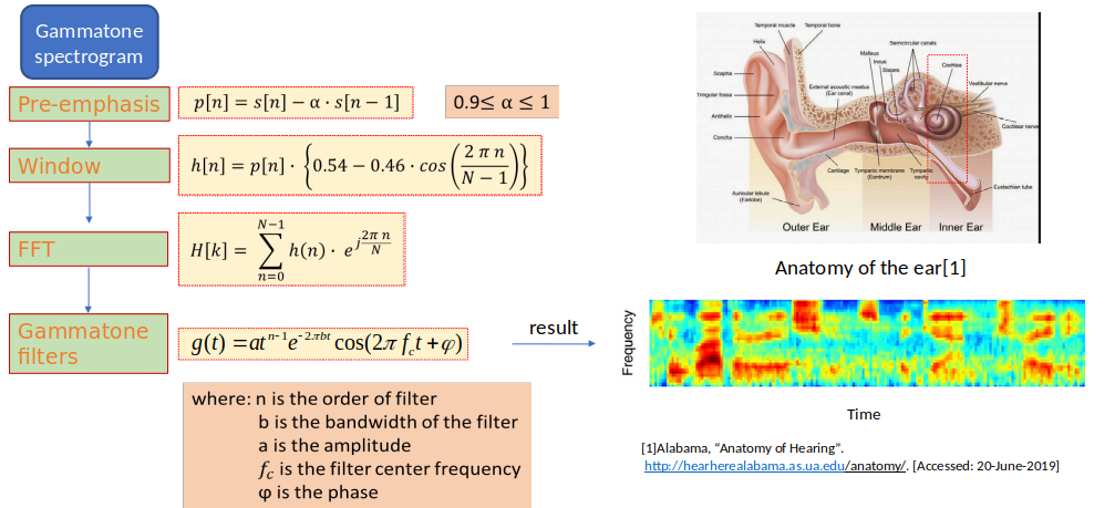
Gammatone Spectrogram Feature:

Gammatone spectrogram is a popular linear approximation to the filtering performed by the ear. This routine provide a simple wrapper for generating time-frequency surfaces based on a gammatone analysis, which can be used as a replacement for a conventional spectrogram. It also provide a fast approximation to this surface based on weighting the output of a conventional FFT.

Convolution Neural Networks (CNNs):

In Neural Networks, Convolution Neural Networks (CNNs) is one of the main categories to do images recognition, images classification. Objects detection, recognition faces,… are some of the areas where CNNs are widely used.

CNN image classification takes an input image, process it and classify it under certain categories (Eg., Bus, Pedestrian, Tram, Metro). Computer sees an input image as array of pixels and it depends on the image resolution. Based on the image resolution, it will see h x w x d (h = Height, w = Width, d = dimension).

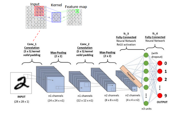
Technically, deep learning CNN models to train and test, each input image will pass it through a series of convolution layers with filters (Kernels), Pooling, fully connected layers (FC) and apply Softmax function to classify an object with probabilistic values between 0 and 1. The above figure is a complete flow of CNN to process an input image and classifies the objects based on values.

(For further information of CNN processes: CNNs)

Data augmentation:

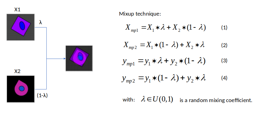
The data augmentation technique called Mixup is extremely efficient at regularizing models in computer vision. As the name kind of suggest, this technique proposes to train the model on a mix of the pictures of the training set. The technique can be described as figure below:

The Baseline Proposal:

This project firstly introduces the baseline proposal:

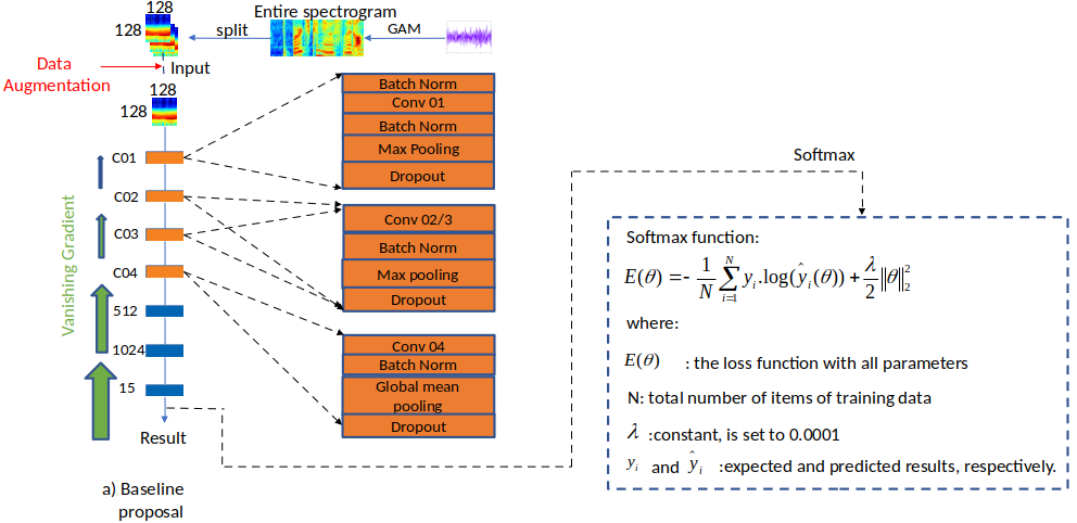
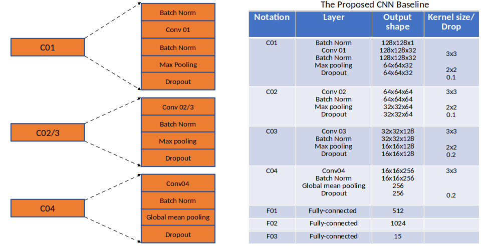
The proposed baseline utilizes Gammatone spectrogram in [22] for the front-end feature extraction. By splitting the entire into patches with the time and frequency resolution of 128x128, these patches are then fed into the back-end classifier. Regarding the back-end process, the proposed model consists of four convolution blocks and three fully connected layers. The first convolution block, denoted as C01, uses batchnorm layers between the input and the output of the convolution layer to speed up the training process and to avoid the Internal Covariate Shift phenomenon [25]. After subsampling the obtained feature maps with a max-pooling layer, the dropout layer is employed for the purpose of preventing over-fitting. The second and the third blocks, denoted as C02 and C03, have a similar structure to C01, a part from no batchnorm layer before convolutional layer. At the convolution block C04, instead of using a max-pooling layer, a global-mean pooling layer is applied to enhance the accuracy since all the spatial regions contribute to the output while the max-pooling layer considers the maximum value of local regions.

The next three fully-connected layers, denoted as F01, F02, and F03, have the role of classification. At the final layer, Softmax function, minimizing the cross-entropy, is applied to tune parameters θ.

The Deeper Training Method:

Inspired by the FreezeOut method suggested by Andrew Brock et al. [26], the training process only trains the hidden layer for a set of portion of the training run, freezes them out one-by-one and excluding them from the backward pass. This project then applies this training method.

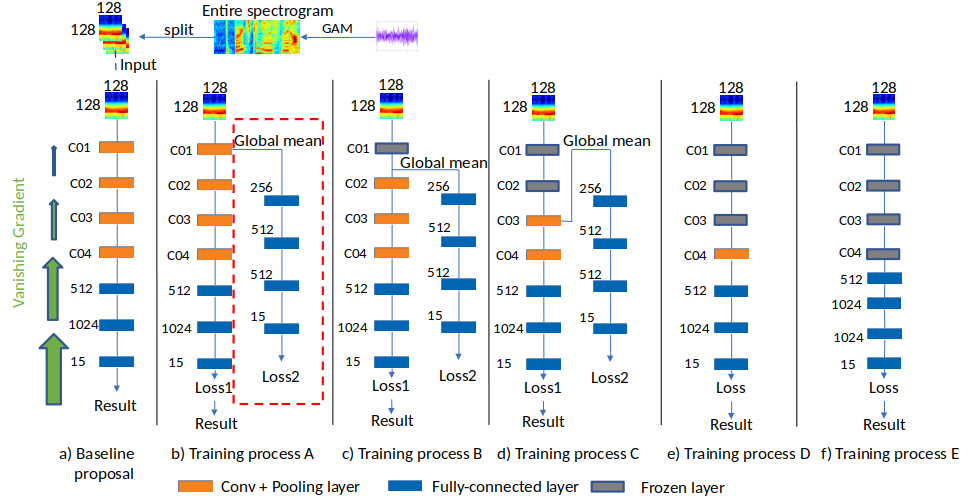
The proposed training process can be separated into five sub-training processes named process A, B, C, D, and E. First, the training process A aims at deeply learning the layer C01 of the baseline. By extracting the global mean of this layer and adding more fully-connected, the model has another loss function that focuses on learning the layer C01. Both loss function use Softmax function and the score is obtained from the original loss function of the baseline proposal. In training process B, the layer C02 is targeted. Therefore, global mean is extracted and fully-connected layers are added to learn this layer while the trainable parameters of layer C01, transferring from the training process A, are remained. Similar to the previous training processes, the C and D deeply learning layers C03 and C04, respectively. Eventually, global mean of the final convolution layer C04 is extracted and goes through a deep neural networks

Experiment Results:

Dataset:

This project exploits the TUT Urban Acoustic Scenes 2016 dataset [24], DCASE2016. As regards the dataset, the audio signals are recorded in six large European cities, in different locations for each scene class. For each recording location, there are 5-6 minutes of audio. The original recordings are split into segments with a length of 30 seconds that are provided in individual files and the sampling frequency is at 44100 Hz. The dataset includes 15 scenes which are Bus, Cafe, Car, City Center, Forest Path, Grocery Store, Home, Lakeside, Beach, Library, Metro Station, Office, Residential Area, Train, Tram, Urban Park.

Baseline Comparison:

The obtained average accuracy over the evaluation set reported by the proposed baseline method and by the DCASE2016 baseline [27] is displayed below:

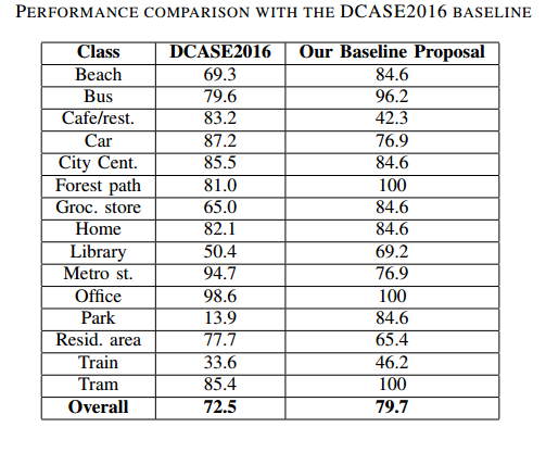
Regarding results over the evaluation set, the classification accuracy on the baseline proposal improves the accuracy by 6% compared to DCASE2016 baseline. Specifically, while the accuracy acquired from the proposed baseline method over park class is significantly higher than from DCASE2016 baseline, the results over Cafe/restaurant of the proposed baseline is much lower.

Experiment Results after Deeper Training Method:

Using mentioned deeper training method above, the overall result are improved by almost 5% compared to the baseline proposal.

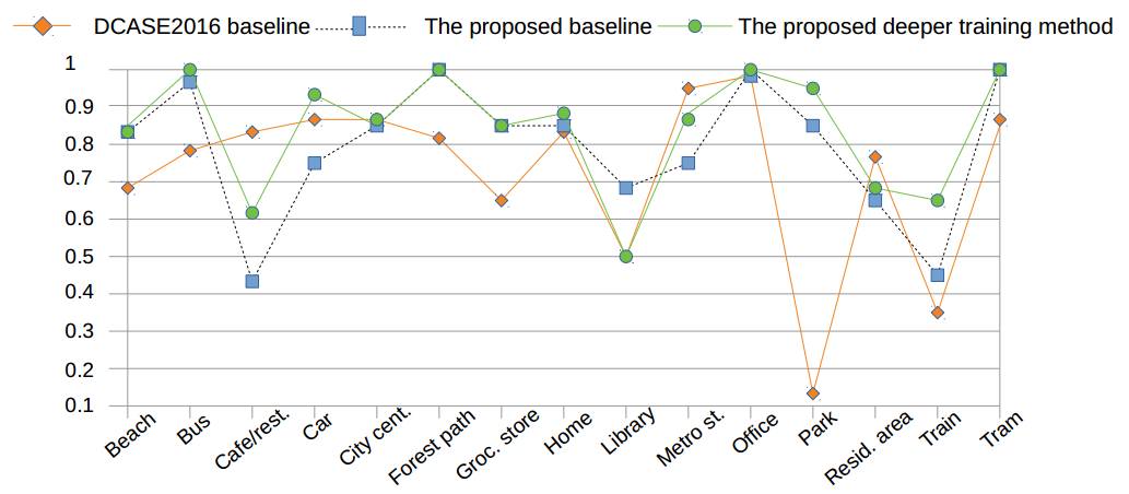
As regards every class, the class accuracy outperforms the baseline proposal, and the deeper training method enhances almost the classification accuracy with the exception of the Library.

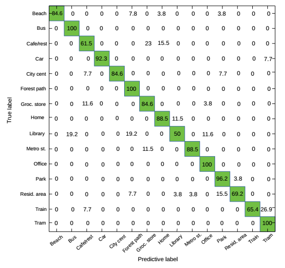
Next, by looking at the confusion matrix, it is able to know which classes are mostly misclassified. These results prove that the proposed model depends more on the background noise than on acoustic event occurrences.

Finally, the overall result of the deeper training method is compared with the results of DCASE2016 challenge (noting that only single classification models are mentioned since plenty of methods show ensemble approach).

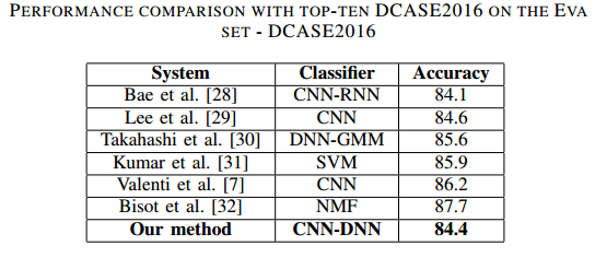
The number in the above table reveals that the best result of the proposed method is very competitive to the top results over the single classification and the CNN approach shows strong classification.

Conclusions

This work has presented a novel deep learning framework for the classification of acoustic scenes. The proposed approach is developed by using on the front-end Gammatone spectrogram and the back-end CNN classification. To deal with implicit challenges in the ASC task, this project investigated that Gammatone spectrogram feature could be effective to compare with other spectrogram features as CQT or log-Mel, and whether applying the deeper training method could improve classification accuracy, allied with the mixup technique.

References

[1] R. F Lyon, “Machine hearing: An emerging field,” IEEE Sig. Proc. Mag., vol. 27, pp. 131–5, 9, 01 2010.

[2] B. N. Schilit, N. Adams, R. Want et al., Context-aware computing applications. Xerox Corporation, Palo Alto Research Center, 1994.

[3] S. Chu, S. Narayanan, C.-C. J. Kuo, and M. J. Mataric, “Where am i? scene recognition for mobile robots using audio features,” in 2006 IEEE International conference on multimedia and expo. IEEE, 2006, pp. 885–888.

[4] T. Heittola, A. Mesaros, A. Eronen, and T. Virtanen, “Context-dependent sound event detection,” EURASIP Journal on Audio, Speech, and Music Processing, vol. 2013, no. 1, p. 1, 2013.

[5] Y. Xu, W. J. Li, and K. K. C. Lee, Intelligent wearable interfaces. Wiley Online Library, 2008.

[6] D. Giannoulis, E. Benetos, D. Stowell, M. Rossignol, M. Lagrange, and M. D. Plumbley, “Detection and classification of acoustic scenes and events: An ieee aasp challenge,” in 2013 IEEE Workshop on Applications of Signal Processing to Audio and Acoustics. IEEE, 2013, pp. 1–4.

[7] M. Valenti, A. Diment, G. Parascandolo, S. Squartini, and T. Virtanen, “Dcase 2016 acoustic scene classification using convolutional neural networks,” in Proc. Workshop Detection Classif. Acoust. Scenes Events, 2016, pp. 95–99.

[8] J.-J. Aucouturier, B. Defreville, and F. Pachet, “The bag-of-frames approach to audio pattern recognition: A sufficient model for urban soundscapes but not for polyphonic music,” The Journal of the Acoustical Society of America, vol. 122, no. 2, pp. 881–891, 2007.

[9] L. Ma, B. Milner, and D. Smith, “Acoustic environment classification,” ACM TASLP, vol. 3, no. 2, pp. 1–22, 2006.

[10] B. Cauchi, “Non-negative matrix factorisation applied to auditory scenes classification,” Master’s thesis, Master ATIAM, Universite Pierre et ´ Marie Curie, 2011.

[11] J. T. Geiger, B. Schuller, and G. Rigoll, “Large-scale audio feature extraction and svm for acoustic scene classification,” in 2013 IEEE WASPAA. IEEE, 2013, pp. 1–4.

[12] F. Itakura, “Line spectrum representation of linear predictor coefficients of speech signals,” The Journal of the Acoustical Society of America, vol. 57, no. S1, pp. S35–S35, 1975.

[13] D. Garcia-Romero and C. Y. Espy-Wilson, “Analysis of i-vector length normalization in speaker recognition systems,” in Twelfth annual conference of the international speech communication association, 2011.

[14] L. Hertel, H. Phan, and A. Mertins, “Classifying variable-length audio files with all-convolutional networks and masked global pooling,” DCASE2016 Challenge, Tech. Rep., September 2016.

[15] A. Rakotomamonjy and G. Gasso, “Histogram of gradients of time–frequency representations for audio scene classification,” IEEE/ACM TASLP, vol. 23, no. 1, pp. 142–153, 2015.

[16] A. J. Eronen, V. T. Peltonen, J. T. Tuomi, A. P. Klapuri, S. Fagerlund, T. Sorsa, G. Lorho, and J. Huopaniemi, “Audio-based context recognition,” IEEE TASLP, vol. 14, no. 1, pp. 321–329, 2006.

[17] O. Gencoglu, T. Virtanen, and H. Huttunen, “Recognition of acoustic events using deep neural networks,” in 2014 22nd EUSIPCO. IEEE, 2014, pp. 506–510.

[18] A. Krizhevsky, I. Sutskever, and G. E. Hinton, “Imagenet classification with deep convolutional neural networks,” in Advances in neural information processing systems, 2012, pp. 1097–1105.

[19] H. Eghbal-Zadeh, B. Lehner, M. Dorfer, and G. Widmer, “Cp-jku submissions for dcase-2016: a hybrid approach using binaural i-vectors and deep convolutional neural networks,” IEEE AASP Challenge on DCASE, 2016.

[20] J. Salamon and J. P. Bello, “Deep convolutional neural networks and data augmentation for environmental sound classification,” IEEE Signal Processing Letters, vol. 24, no. 3, pp. 279–283, 2017.

[21] R. Lu, Z. Duan, and C. Zhang, “Metric learning based data augmentation for environmental sound classification,” in 2017 IEEE WASPAA. IEEE, 2017, pp. 1–5.

[22] J. Dennis, Q. Yu, H. Tang, H. D. Tran, and H. Li, “Temporal coding of local spectrogram features for robust sound recognition,” in 2013 IEEE International Conference on Acoustics, Speech and Signal Processing. IEEE, 2013, pp. 803–807.

[23] A. Diment and T. Virtanen, “Transfer learning of weakly labelled audio,” in 2017 ieee waspaa. IEEE, 2017, pp. 6–10.

[24] A. Mesaros, T. Heittola, and T. Virtanen, “Tut database for acoustic scene classification and sound event detection,” in 2016 24th EUSIPCO. IEEE, 2016, pp. 1128–1132.

[25] S. Ioffe and C. Szegedy, “Batch normalization: Accelerating deep network training by reducing internal covariate shift,” arXiv preprint arXiv:1502.03167, 2015.

[26] A. Brock, T. Lim, J. M. Ritchie, and N. Weston, “Freezeout: Accelerate training by progressively freezing layers,” arXiv preprint arXiv:1706.04983, 2017.

[27] A. Mesaros, T. Heittola, E. Benetos, P. Foster, M. Lagrange, T. Virtanen, and M. D. Plumbley, “Detection and classification of acoustic scenes and events: Outcome of the dcase 2016 challenge,” IEEE/ACM TASLP, vol. 26, no. 2, pp. 379–393, 2018.

[28] S. H. Bae, I. Choi, and N. S. Kim, “Acoustic scene classification using parallel combination of lstm and cnn,” in Proceedings of the DCASE2016, 2016, pp. 11–15.

[29] Y. Han and K. Lee, “Convolutional neural network with multiple-width frequency-delta data augmentation for acoustic scene classification,” IEEE AASP Challenge on DCASE, 2016.

[30] G. Takahashi, T. Yamada, S. Makino, and N. Ono, “Acoustic scene classification using deep neural network and frame-concatenated acoustic feature,” Detection and Classification of Acoustic Scenes and Events, 2016.

[31] B. Elizalde, A. Kumar, A. Shah, R. Badlani, E. Vincent, B. Raj, and I. Lane, “Experiments on the dcase challenge 2016: Acoustic scene classification and sound event detection in real life recording,” arXiv preprint arXiv:1607.06706, 2016.

[32] V. Bisot, R. Serizel, S. Essid, and G. Richard, “Supervised nonnegative matrix factorization for acoustic scene classification,” IEEE AASP Challenge on DCASE, p. 27, 2016.